Why does changing the number of heads not change the number of parameters in the model? – That was the question i was asking myself. After drawing out the matrix multiplication and having gained the insight, i’d like to share this knowledge and try to visually explain the Multi Head Attention (MHA) mechanism on a tiny example. Take note that i will only go through the MHA, as there are already excellent explanations to the Transformer model out there such as the one from Jay Alammar (The Illustrated Transformer).
Observation: Changing the number of heads does not change the number of parameters
from transformers import RobertaForMaskedLM, RobertaConfig

config_3 = RobertaConfig( num_attention_heads=4)
config_12 = RobertaConfig(num_attention_heads=12)

model_head3 = RobertaForMaskedLM(config=config_3)
model_head12 = RobertaForMaskedLM(config=config_12)

print(f"Number of parameters with 3 heads:{sum(p.numel() for p in model_head3.parameters() if p.requires_grad)}")
print(f"Number of parameters with 12 heads:{sum(p.numel() for p in model_head12.parameters() if p.requires_grad)}")

# output:
# Number of parameters with 3 heads:109514298
# Number of parameters with 12 heads:109514298
I noticed, that even though the number of heads changed, the number of parameters in the model stayed the same. So why is that so?
In-Depth Visual Explanation of Multi Head Attention
In the following section we will be only focusing on the Multi Head Attention part of Vaswani et al. (2017)’s Attention Is All You Need paper. To get started with this topic, i will be relying on the illustrations of Jay Alammar
Self-Attention
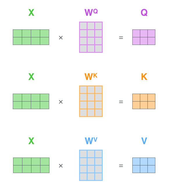
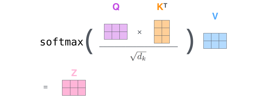
The embeddings (X) are multiplied with weight matrices WQ. WK, WV to generate the Queries (Q), Keys (K) and Values (V) respectively. Afterwards, those matrices Q, K and V are “mixed” together to obtain the self attention matrix (Z).
Multi-Head
“Instead of performing a single attention function with d_model-dimensional keys, values and queries, we found it beneficial to linearly project the queries, keys and values h times with different, learned linear projections to d_k, d_k and d_v dimensions, respectively.” (Vaswani et al, 2017, p.4)

This means, that the embedding X is not just multiplied once with the weight matrices WQ, WK, WV to create Q, K and V but rather with h different weight matrices WQ_i, WK_i, WV_i. The parameters are listed as following:
- h : number of heads
- d_model : is the size of the dimension of the embedding
- d_k : is the size of the dimension of the queries and keys
- d_v: is the size of the dimension of the value, thus theoretically d_v could be different than d_k.
- d_k = d_v = d_model/h
The following illustration shall shed some light, by simulating one linear projection of an embedding with different number of heads. Take note, that with the changing number of heads, d_k and d_v do change and thus the dimensionality of the weight matrices. This is also the reason, why the dimension of the embeddings have to be a multiple of the number of heads – because of maths 🙂
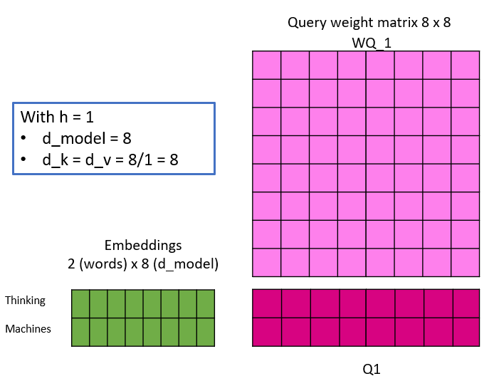
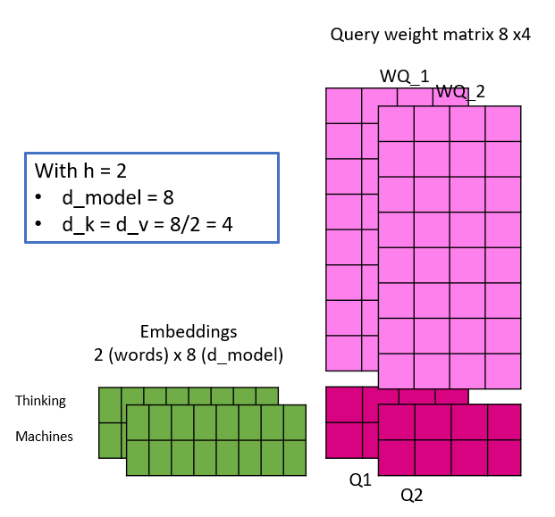
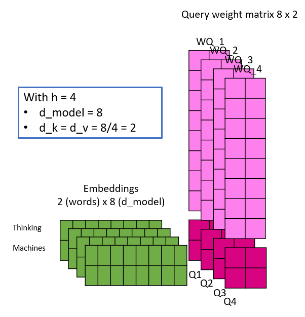
The Keys, Queries and Values are calculated as illustrated and the attention matrix Z is then calculated for each head in parallel. Evidently, by changing the number of heads, the number of weight parameters do not change, as observed initially.
For me it was important to understand, that although the number of heads change, the input embeddings are not split but rather copied and each one of those copies is multiplied by different weight matrices (heads) to calculate the respective Queries, Keys and Values.
“Multi-head attention allows the model to jointly attend to information from different representation subspaces at different positions” (Vaswani et al., 2017, p.5)
Each head is responsible to fully calculate the attention for the whole embedding, not just for a subset of it and creates h attention matrices. As quoted, these matrices allow to attend to information from different angles. I remember having read an insightful comment, that those can be compared to feature maps in object detection, which also just attend for a specific information pattern.
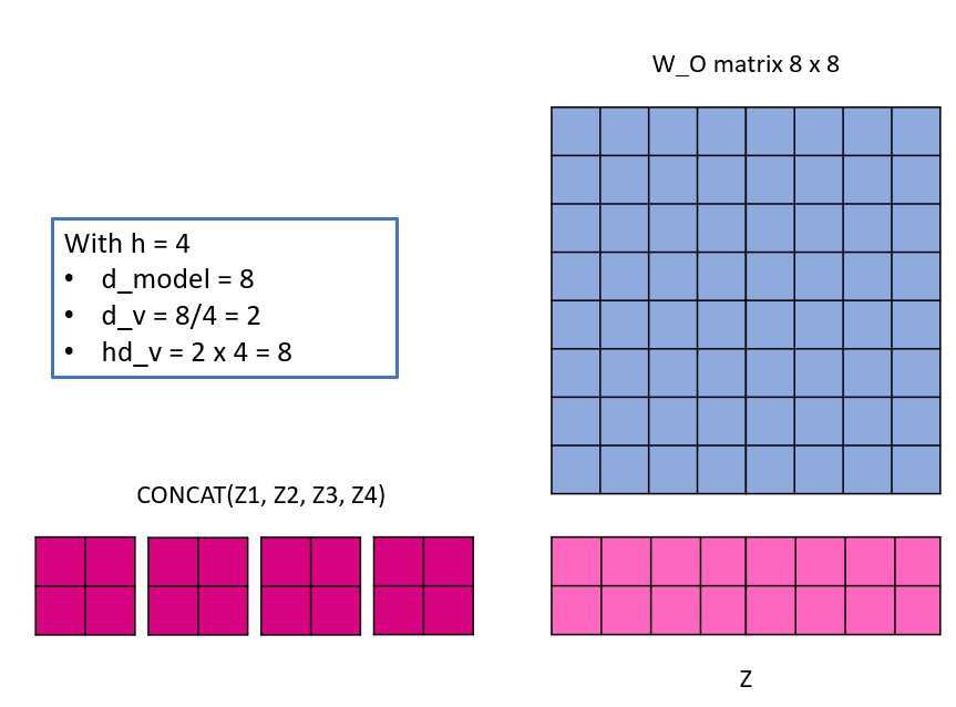
Finally, because a single matrix is expected, the multiple h attention matrices now need to be squished together. This is done by concatinating them and then multiplying them one last time with a weight matrix W_O, with dimensions hd_v x d_model.
References
Vaswani, A., Shazeer, N., Parmar, N., Uszkoreit, J., Jones, L., Gomez, A. N., Kaiser, L., & Polosukhin, I. (2017). Attention Is All You Need. ArXiv:1706.03762 [Cs]. http://arxiv.org/abs/1706.03762
Further Readings
- BERT Research – Ep. 6 – Inner Workings III – Multi-Headed Attention, a very insightful video, which also goes through Jay Alammars post in depth, however was just short in explaining the impact of changing the number of attention heads.
- How to account for the no:of parameters in the Multihead self-Attention layer of BERT – stackexchange, Dileep Kumar Patchigolla explains how he calculated the number of weight parameters with regards to the Multi Head Attention part